Reapply existing signatures

Simple example of fitting the provided example data to the 5 ES model. In this example, we load some abundance data provided in cvanmf using the data.example_abundance() function. This provides the data as a pandas DataFrame, with each row being a feature (in this case a bacterial genus) and each column a sample. If you are using your own data, you will first need to load it using pandas, typically via read_csv.

from cvanmf import models, data
import numpy as np

# The example data is quite large, so we'll take a subset of samples
result = models.five_es().reapply(
    # The input should be as a pandas DataFrame, with features on rows and
    # samples on columns. Data does not need to be normalised in this case,
    # the `reapply` method of the `five_es` object will apply the appropriate
    # transformations.
    y=data.example_abundance().iloc[:, :30]
)

result.model_fit.describe()

WARNING [cvanmf.models] [15/04/2026 10:41:50]: If you use the 5ES model please cite Frioux, C. et al. Enterosignatures define common bacterial guilds in the human gut microbiome. Cell Host & Microbe 31, 1111-1125.e6 (2023). https://doi.org/10.1016/j.chom.2023.05.024

count    30.000000
mean      0.797996
std       0.185145
min       0.203682
25%       0.763434
50%       0.862407
75%       0.930804
max       0.974751
Name: model_fit, dtype: float64

The reapply method on one of the existing models in the models package often includes method to normalise and process the data into the correct format. For the five_es model this includes normalising to relative abundance, and attempting to match the names of taxa between input and the model. Check the description of each more in the API reference for details.

The results object is a Decomposition class object. The Enterosignature weights for each sample are in the H matrix of the results object.

result.h.head().iloc[:, :5]

	W2.35.ST	W1.41.ST	W2.42.ST	W1.39.ST	M1.61.ST
ES_Bact	1.088325e-03	0.000057	5.533855e-06	2.797162e-15	5.123730e-07
ES_Bifi	2.782562e-08	0.000582	2.067819e-03	6.447965e-03	9.524048e-05
ES_Esch	7.382243e-04	0.000032	1.588800e-02	1.233557e-03	4.232990e-03
ES_Prev	1.778084e-02	0.037536	3.071650e-02	2.887819e-02	3.282901e-02
ES_Firm	1.282287e-02	0.004567	2.772057e-15	5.027370e-03	4.772470e-03

We can get a scaled version of the H matrix (so each sample sums to 1), and visualise this using a mix of the inbuilt methods.

assert np.allclose(result.scaled('h').sum(), 1.0)
result.scaled('h').iloc[:, :5]

	W2.35.ST	W1.41.ST	W2.42.ST	W1.39.ST	M1.61.ST
ES_Bact	3.355890e-02	0.001341	1.136832e-04	6.726035e-14	0.000012
ES_Bifi	8.580131e-07	0.013607	4.247966e-02	1.550473e-01	0.002271
ES_Esch	2.276342e-02	0.000748	3.263907e-01	2.966203e-02	0.100953
ES_Prev	5.482788e-01	0.877526	6.310159e-01	6.944029e-01	0.782944
ES_Firm	3.953980e-01	0.106778	5.694698e-14	1.208878e-01	0.113819

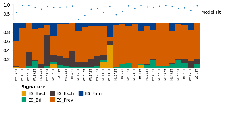
The relative weights can be plotted as a stacked bar, using the plot_relative_weight method. By default, the top part of this plot shows the model fit of each sample (the cosine angle between the sample and X and in WH), with 1 being good and 0 bad. A default line of 0.4 for “poor model fit” is given, based on the Enterosignatures paper. Below this is a stacked bar plot, showing the relative abundance of each signature in each sample.

Most plots in the package are produced using plotnine. plot_relative_weight uses Marsilea instead, as the options for combining multiple plotnine plots are currently limitted. The object returned is a WhiteBoard object, which has a method render() which can be used to display the plot.

# The heights parameter controls the relative height of each components
result.plot_relative_weight(heights=[0.5, 0.7, 0.25], width=6, height=3, sample_label_size=6).render()

Examples of extra visualisations can be found in the “De-novo signatures” section.