De-novo signatures

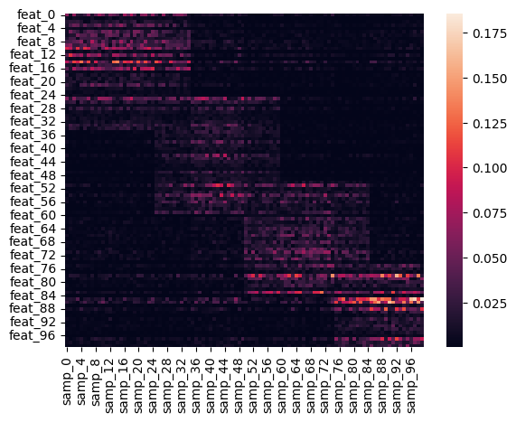
We can attempt to discover signatures from new data. For these examples we will use a simple synthetic dataset with 4 signatures which slightly overlap.

import seaborn as sns
import pathlib
from cvanmf.denovo import rank_selection, plot_rank_selection, decompositions, Decomposition
from cvanmf import models, data

blocks = data.synthetic_blocks(
    overlap=0.4, 
    k=4, 
    scale_lognormal_params=dict(sigma=0.75)
)
blocks
# Each feature is assigned a weight drawn from a lognormal distribution, to roughly simulate some features (such a taxon) 
# generally taking higher values in input data.

Synthetic Overlapping Blocks
cvanmf example data
shape	(100, 100)
rank	4
description	Synthetic data with blocks along the diagonal which overlap to a defined extent.
doi
citation

Data generated or provided in the data module is provided as a named tuple containing description and metadata, as well as the data. The dataframe can be accessed as x.data

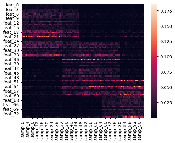
x = blocks.data
sns.heatmap(blocks.data)

<Axes: >

Rank selection

The number of ranks \(k\) is unknown, however we can attempt to estimate it using bi-crossvalidation. This tries learning a held out part of the data using the other parts for a range of ranks a large number of times, and we look at measures of how well the held out part was estimated to identify a suitable rank. These are run from largest rank to smallest, so the estimate of time tends to start of conservative.

rank_sel_res = rank_selection(x=x, ranks=range(2, 7), shuffles=20, seed=4298, progress_bar=False)
# shuffles sets the number iterations of bi-crossvalidation which are run. 
# The default is 100, it has been set lower here to make the documentation easier to compile, but 100 is a more 
# sensible value for real data

plot_rank_selection(rank_sel_res, jitter=False, n_col=3)

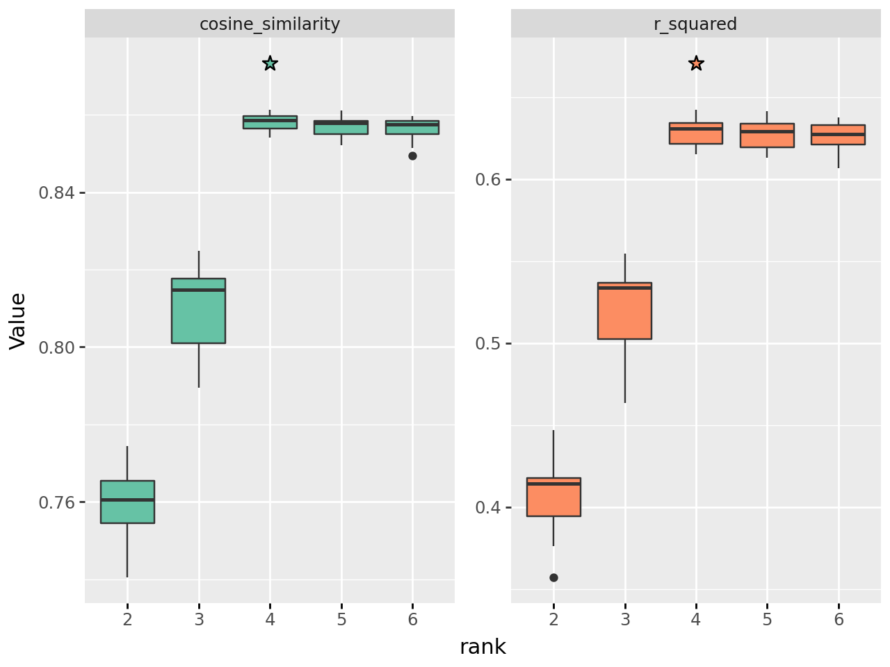
In these plots you are typically looking for elbow points; ranks after which the quality of the decomposition does not improve as rapidly, suggesting that adding more signatures is no longer contributing much explanatory power.

In our example, cosine similarity increases rapidly until \(k=4\) where the rate of increase slows, indicating this is a suitable rank. Real world examples will rarely be so clear, and often several ranks will appear suitable.

The different measures here are:

• Cosine Similarity: Higher is better. The angle between the true data and estimated data, considering each as a flattened 1d vector

• L2 Norm: Euclidean distance between true and estimated data. Lower is better.

• R-squared: Coefficient of determination between true and estimated data. Higher is better.

• Reconstruction Error: Measure of the error in the estimated data compared to true. Lower is better.

• Residual Sum of Sqaures: Lower is better

• Sparsity H: Sparsity of the H matrix

• Sparsity W: Sparsity of the W matrix

When there are several candidate ranks, it is useful to generate decompositions for each and manually inspect them. This is usually the case, and some researcher judgement is required in eventually selecting which rank decomposition to use.

Regularisation selection

Background

\(L1\) regularisation can be applied to encourage sparsity in the decomposition (fewer entries in \(W\) and \(H\) with high values). A sparse solution can have benefits for intuitive understanding, for instance if we are decomposing a table of genes, a signature with high weights for a few genes, rather than lower weights for many genes, can be easier to interpret biologically.

\(L2\) regularisation instead encourages a more even distribution of weights across in both \(W\) and \(H\), leading to more evenly distributed weights and lower sparsity.

The degree of regularisation is controlled by two parameters, \(l1\_ratio\) and \(alpha\) from the underlying NMF implementation we use from scikit-learn. Currently regularisation is applied to both the \(H\) and \(W\) matrices, though sklearn supports only applying to one.

• \(l1\_ratio\) - Between 0 and 1, with 1 applying only \(L1\) regularisation, and 0 applying only \(L2\) regularisation, and any value between being a mix.

• \(alpha\) - Regularisation coefficient. A value of 0 means applying no regularisation. By default when selecting an \(alpha\) parameter, cvanmf will try values \(2^i\) for \(i \in \{-5, -4, \dots, 2\}\)

Application

We give an example here of \(L1\) regularisation to encourage sparsity. cvanmf provides the function regu_selection to test values of \(alpha\) for a given \(l1\_ratio\). As we want a sparse solution, we will use \(l1\_ratio = 1\). The function only accepts one rank, we have to have already selected the rank of decomposition we want.

from cvanmf.denovo import regu_selection, plot_regu_selection

best_alpha, regu_sel_res = regu_selection(x=x, rank=4, shuffles=10, seed=4298, l1_ratio=1.0, progress_bar=False)
# shuffles sets the number iterations of bi-crossvalidation which are run. 
# The default is 100, it has been set lower here to make the documentation easier to compile, but 100 is a more 
# sensible value for real data

best_alpha

0.0003125

plot_regu_selection(regu_sel_res)

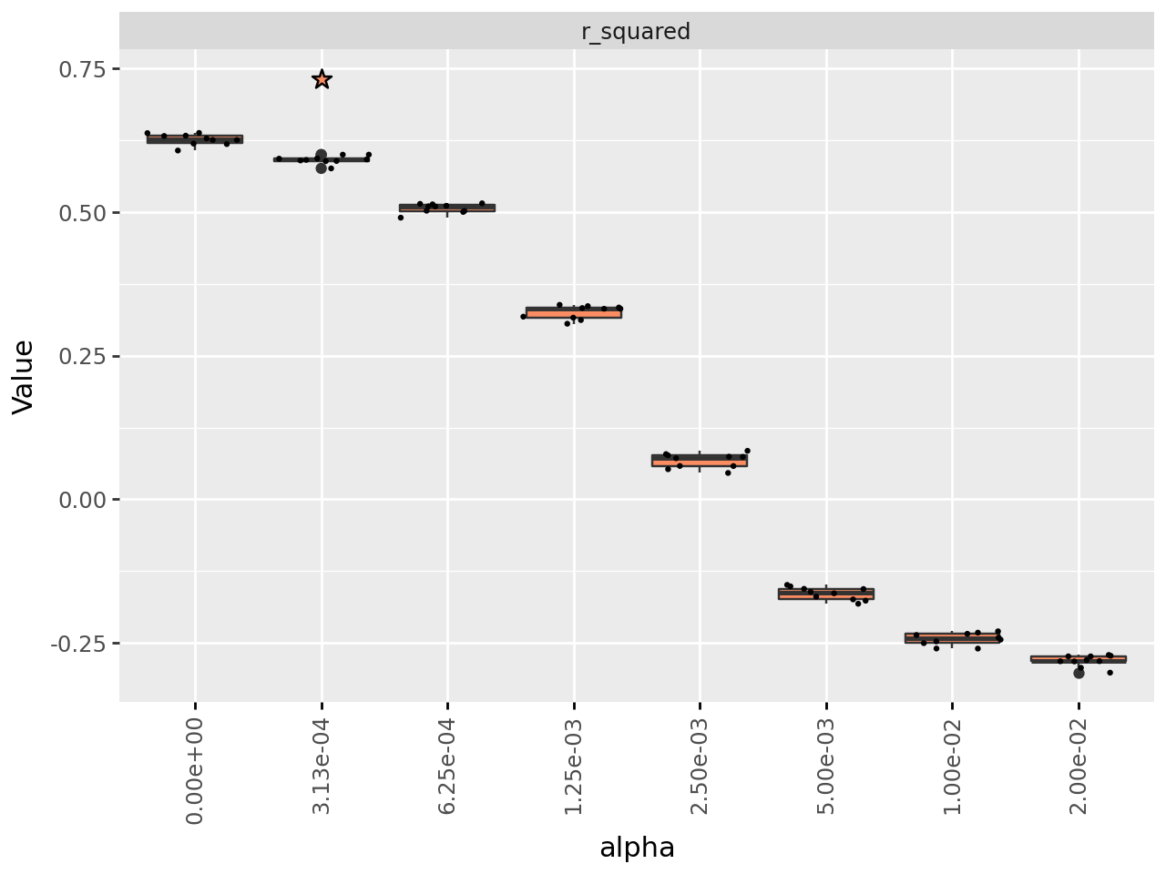
A higher value of alpha leads to greater sparsity, although in this case not by much until high values of \(alpha\). However, the measure of how well the decomposition reconstructs the input data also monotonically decrease as \(alpha\) increases. cvanmf by default identifies the tested value of \(alpha\) for which the \(R^2\) is not significantly worse than \(alpha=0\), which is returned as the first element of the results.

best_alpha

0.0003125

Generating decompositions

For the ranks of interest, we can generate several decompositions to investigate. NMF solutions are non-unique and depend on the initialisation of the \(H\) and \(W\) matrices; some initialisations may give a better solution than others. One approach is to make many decompositions, and select those which optimise some criteria, such as reconstruction error.

Here we make 100 decompositions for each of ranks 3, 4, and 5, and keep only the top 5 for each rank. The result is a dictionary, with the key being the rank, and the value a list of Decompositions with the first being the best (lowest reconstruction error).

decomps = decompositions(x, ranks=[3, 4, 5], top_n=5, random_starts=5, seed=4928, progress_bar=False)
# or to use regularisation
# decomps = decompositions(x, ranks=[3, 4, 5], top_n=5, random_starts=5, seed=4928, l1_ratio=1.0, alpha=best_alpha)
decomps

{3: [Decomposition[rank=3, beta_divergence=23.4],
  Decomposition[rank=3, beta_divergence=23.4],
  Decomposition[rank=3, beta_divergence=23.4],
  Decomposition[rank=3, beta_divergence=23.5],
  Decomposition[rank=3, beta_divergence=23.5]],
 4: [Decomposition[rank=4, beta_divergence=16.7],
  Decomposition[rank=4, beta_divergence=16.7],
  Decomposition[rank=4, beta_divergence=16.7],
  Decomposition[rank=4, beta_divergence=16.7],
  Decomposition[rank=4, beta_divergence=16.7]],
 5: [Decomposition[rank=5, beta_divergence=15.8],
  Decomposition[rank=5, beta_divergence=15.8],
  Decomposition[rank=5, beta_divergence=15.8],
  Decomposition[rank=5, beta_divergence=15.9],
  Decomposition[rank=5, beta_divergence=15.9]]}

You can use regularisation parameters here, but be aware the than same \(alpha\) is applied to all ranks, which may not be suitable as \(alpha\) is selected for a decomposition of specific rank.

We can inspect the decompositions using some inbuilt plotting functions

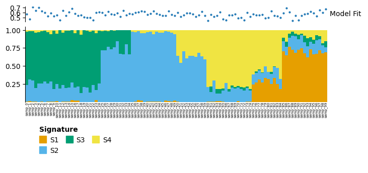
decomps[4][0].plot_relative_weight(heights=[0.3, 1, 0.2]).render()

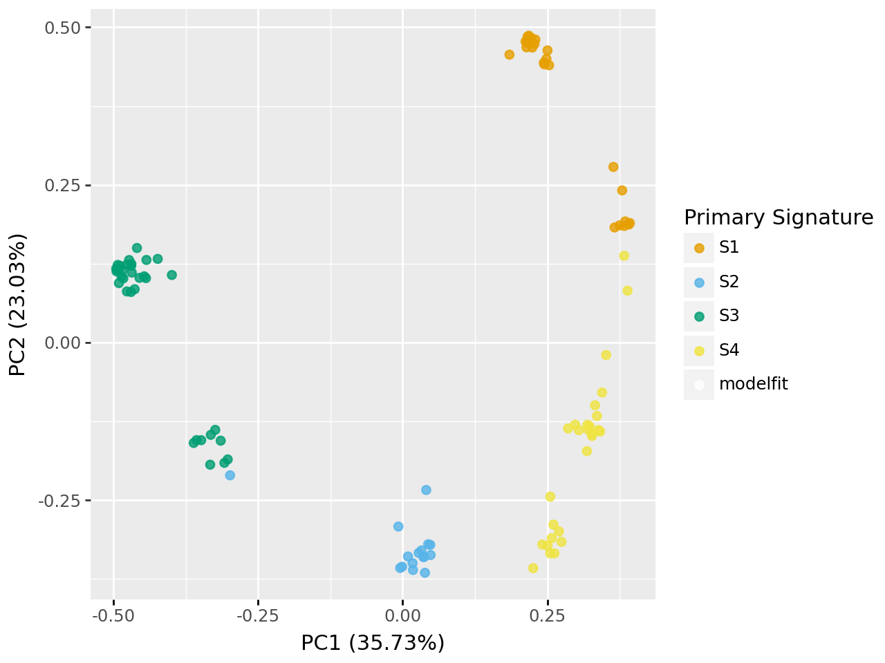
decomps[4][0].plot_pcoa()

/home/docs/checkouts/readthedocs.org/user_builds/cvanmf/envs/latest/lib/python3.12/site-packages/skbio/stats/ordination/_principal_coordinate_analysis.py:476: UserWarning: 'where' used without 'out', expect unitialized memory in output. If this is intentional, use out=None.

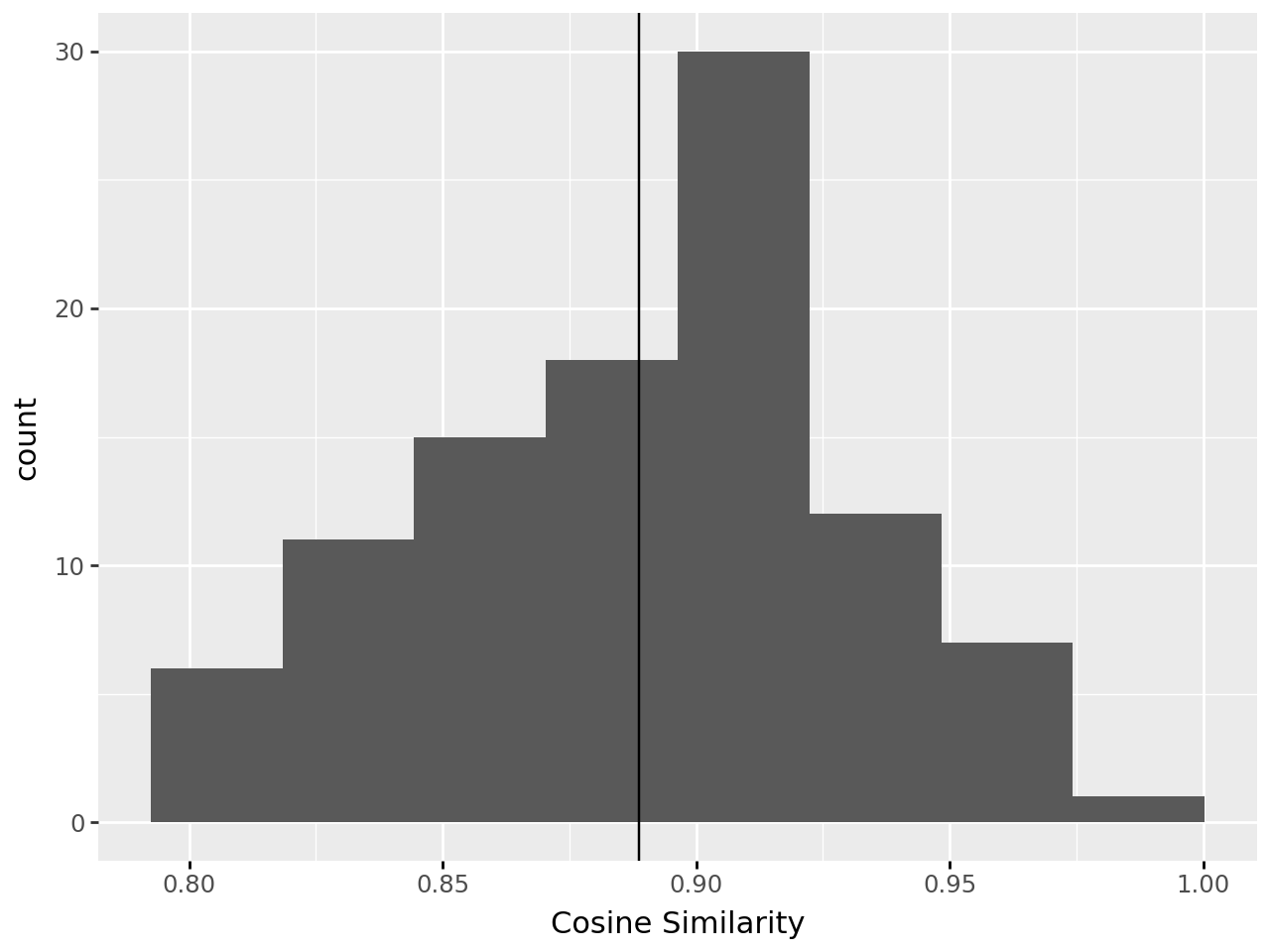
decomps[4][0].plot_modelfit()

/home/docs/checkouts/readthedocs.org/user_builds/cvanmf/envs/latest/lib/python3.12/site-packages/plotnine/stats/stat_bin.py:109: PlotnineWarning: 'stat_bin()' using 'bins = 8'. Pick better value with 'binwidth'.

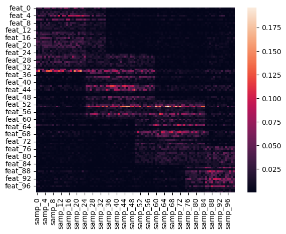
decomps[4][0].plot_feature_weight()

Reapplying this model

Now that we have generated a model, we can reapply it to new data. We’ll make two datasets:

• y_similar: Has exactly the same properties as our original X. The model should describe this well.

• y_different: Has fewer features, and different number of blocks, so should handle this poorly.

y_similar = data.synthetic_blocks(
    overlap=0.4, 
    k=4, 
    scale_lognormal_params=dict(sigma=0.75)
).data
sns.heatmap(y_similar)

<Axes: >

y_different = data.synthetic_blocks(
    m=75,
    overlap=0.4, 
    k=3, 
    scale_lognormal_params=dict(sigma=0.75)
).data
sns.heatmap(y_different)

<Axes: >

Applying our existing model to the data is simple…

d_similar = decomps[4][0].reapply(
    y=y_similar
)
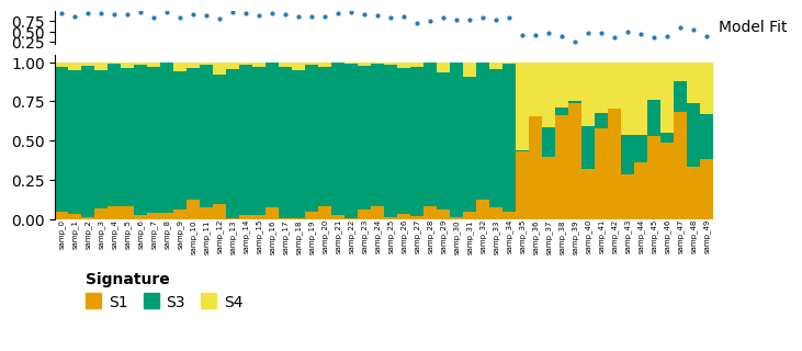
d_similar.plot_relative_weight(heights=[0.3, 1, 0.2]).render()

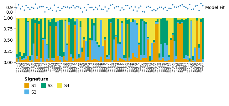
For the similar data, the model looks to have described the data reasonably well, with overlapping blocks of signatures.

d_different = decomps[4][0].reapply(
    y=y_different
)
d_different.plot_relative_weight(heights=[0.3, 1, 0.2]).render()

For dissimilar data is has still performed okay. If we look at the decomposition, we can see that to align the data cvanmf has removed from the signature weight matrix and features which are not in the new data (y_different), so only 75 features are used here.

decomps[4][0].w.loc[d_different.w.index] == d_different.w

	S1	S2	S3	S4
feat_0	True	True	True	True
feat_1	True	True	True	True
feat_2	True	True	True	True
feat_3	True	True	True	True
feat_4	True	True	True	True
...	...	...	...	...
feat_70	True	True	True	True
feat_71	True	True	True	True
feat_72	True	True	True	True
feat_73	True	True	True	True
feat_74	True	True	True	True

75 rows × 4 columns

Slicing decompositions

We might be interested in visualising or analysis only a subset of a decomposition; perhaps we only want to look at one cohort of samples in a model, or only at some of the signatures. Decomposition objects can be indexed by sample, feature, and signature in that order. Normal slice syntax (1:5), lists of index names, or lists of index positions are supported. You can supply a mix of these.

This can also be used for abitrary reordering of samples and features for visualisations.

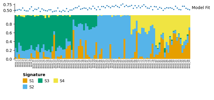
decomp_slcd = decomps[4][0][:50, :, ["S1", "S3", "S4"]]
decomp_slcd.plot_relative_weight(heights=[0.3, 1, 0.2]).render()

Here we have restricted to just the first 50 samples, and only signatures S1, S3 and S4. In the full decomposition, S2is important to described many samples from samp_35 to samp_49, so the model fit for these is much poorer in this reduced model.

Another potential use for the slicing syntax is to reorder samples based on some metadata condition. The method is illustrated below with a random reordering.

# Reorder samples - here we're just generating a random order
import random
new_order = list(range(decomps[4][0].h.shape[1]))
random.shuffle(new_order)

# Reorder the decomposition
decomps[4][0][new_order].plot_relative_weight(heights=[0.3, 1, 0.2]).render()

Saving and loading

Decompositions can be saved to disk for analysis in other environments, or saved and reloaded later.

Decomposition.save_decompositions(decomps, output_dir=pathlib.Path("test_save"), symlink=False, plots=False)
# We're not writing any plots here (as they take some time), but you can set this to
# - True: make all plots
# - List of plots names: make all the listed plots
# - None: Make all plots, unless there are many samples (>250), in which case omit any plots which have an element for each sample

! ls test_save/**/**

test_save/3/0:
h.tsv			  parameters.yaml	 representative_signatures.tsv
h_scaled.tsv		  primary_signature.tsv  w.tsv
model_fit.tsv		  properties.yaml	 w_scaled.tsv
monodominant_samples.tsv  quality_series.tsv	 x.tsv

test_save/3/1:
h.tsv			  parameters.yaml	 representative_signatures.tsv
h_scaled.tsv		  primary_signature.tsv  w.tsv
model_fit.tsv		  properties.yaml	 w_scaled.tsv
monodominant_samples.tsv  quality_series.tsv	 x.tsv

test_save/3/2:
h.tsv			  parameters.yaml	 representative_signatures.tsv
h_scaled.tsv		  primary_signature.tsv  w.tsv
model_fit.tsv		  properties.yaml	 w_scaled.tsv
monodominant_samples.tsv  quality_series.tsv	 x.tsv

test_save/3/3:
h.tsv			  parameters.yaml	 representative_signatures.tsv
h_scaled.tsv		  primary_signature.tsv  w.tsv
model_fit.tsv		  properties.yaml	 w_scaled.tsv
monodominant_samples.tsv  quality_series.tsv	 x.tsv

test_save/3/4:
h.tsv			  parameters.yaml	 representative_signatures.tsv
h_scaled.tsv		  primary_signature.tsv  w.tsv
model_fit.tsv		  properties.yaml	 w_scaled.tsv
monodominant_samples.tsv  quality_series.tsv	 x.tsv

test_save/4/0:
h.tsv			  parameters.yaml	 representative_signatures.tsv
h_scaled.tsv		  primary_signature.tsv  w.tsv
model_fit.tsv		  properties.yaml	 w_scaled.tsv
monodominant_samples.tsv  quality_series.tsv	 x.tsv

test_save/4/1:
h.tsv			  parameters.yaml	 representative_signatures.tsv
h_scaled.tsv		  primary_signature.tsv  w.tsv
model_fit.tsv		  properties.yaml	 w_scaled.tsv
monodominant_samples.tsv  quality_series.tsv	 x.tsv

test_save/4/2:
h.tsv			  parameters.yaml	 representative_signatures.tsv
h_scaled.tsv		  primary_signature.tsv  w.tsv
model_fit.tsv		  properties.yaml	 w_scaled.tsv
monodominant_samples.tsv  quality_series.tsv	 x.tsv

test_save/4/3:
h.tsv			  parameters.yaml	 representative_signatures.tsv
h_scaled.tsv		  primary_signature.tsv  w.tsv
model_fit.tsv		  properties.yaml	 w_scaled.tsv
monodominant_samples.tsv  quality_series.tsv	 x.tsv

test_save/4/4:
h.tsv			  parameters.yaml	 representative_signatures.tsv
h_scaled.tsv		  primary_signature.tsv  w.tsv
model_fit.tsv		  properties.yaml	 w_scaled.tsv
monodominant_samples.tsv  quality_series.tsv	 x.tsv

test_save/5/0:
h.tsv			  parameters.yaml	 representative_signatures.tsv
h_scaled.tsv		  primary_signature.tsv  w.tsv
model_fit.tsv		  properties.yaml	 w_scaled.tsv
monodominant_samples.tsv  quality_series.tsv	 x.tsv

test_save/5/1:
h.tsv			  parameters.yaml	 representative_signatures.tsv
h_scaled.tsv		  primary_signature.tsv  w.tsv
model_fit.tsv		  properties.yaml	 w_scaled.tsv
monodominant_samples.tsv  quality_series.tsv	 x.tsv

test_save/5/2:
h.tsv			  parameters.yaml	 representative_signatures.tsv
h_scaled.tsv		  primary_signature.tsv  w.tsv
model_fit.tsv		  properties.yaml	 w_scaled.tsv
monodominant_samples.tsv  quality_series.tsv	 x.tsv

test_save/5/3:
h.tsv			  parameters.yaml	 representative_signatures.tsv
h_scaled.tsv		  primary_signature.tsv  w.tsv
model_fit.tsv		  properties.yaml	 w_scaled.tsv
monodominant_samples.tsv  quality_series.tsv	 x.tsv

test_save/5/4:
h.tsv			  parameters.yaml	 representative_signatures.tsv
h_scaled.tsv		  primary_signature.tsv  w.tsv
model_fit.tsv		  properties.yaml	 w_scaled.tsv
monodominant_samples.tsv  quality_series.tsv	 x.tsv

These decompositions can be loaded from disk again

loaded_decomps = Decomposition.load_decompositions(in_dir=pathlib.Path("test_save"))
loaded_decomps

{3: [Decomposition[rank=3, beta_divergence=23.4],
  Decomposition[rank=3, beta_divergence=23.4],
  Decomposition[rank=3, beta_divergence=23.4],
  Decomposition[rank=3, beta_divergence=23.5],
  Decomposition[rank=3, beta_divergence=23.5]],
 4: [Decomposition[rank=4, beta_divergence=16.7],
  Decomposition[rank=4, beta_divergence=16.7],
  Decomposition[rank=4, beta_divergence=16.7],
  Decomposition[rank=4, beta_divergence=16.7],
  Decomposition[rank=4, beta_divergence=16.7]],
 5: [Decomposition[rank=5, beta_divergence=15.8],
  Decomposition[rank=5, beta_divergence=15.8],
  Decomposition[rank=5, beta_divergence=15.8],
  Decomposition[rank=5, beta_divergence=15.9],
  Decomposition[rank=5, beta_divergence=15.9]]}

An individual decomposition can also be loaded

one_decomp = Decomposition.load(in_dir=pathlib.Path("test_save/5/0/"))
one_decomp

Decomposition[rank=5, beta_divergence=15.8]

! rm -rf test_save

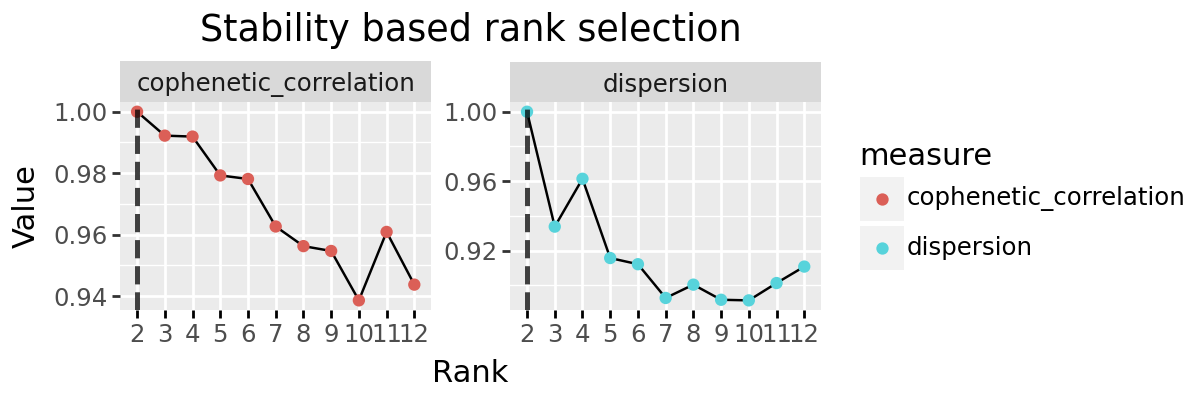
Stability based rank selection

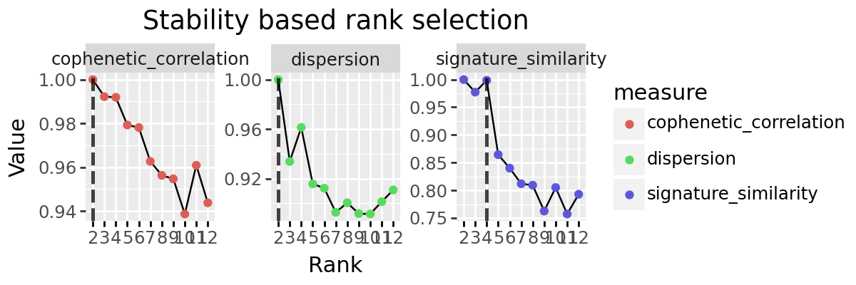
We implement to other popular methods for rank selection, the cophenetic correlation and dispersion coefficients. These are both based on the stability of discrete clusting provided by the decomposition. Each sample (or feature) is ‘assigned’ to the signature for which it has maximum weight, and a consensus matrix created indicating which pairs of elements are found assigned to the same signature. How similar these consensus matrices are is evaluated across multiple random initialisations, with the intuition that a good factorisation should be stable across intitialisation conditions.

We implement these with the functions cophenetic_correlation, dispersion, and plot_stability_rank_selection.

Making decompositions with random intialisations

The first step is to make a number of decompositions for each rank of interest using decompositions. We are using 10 here, but more (100) would be good for real experiments. The initialisation method should be one which includes a random factor, so either random or nndssvdar.

rs_decomps = decompositions(x, ranks=[2, 3, 4, 5, 6, 7, 8, 9, 10, 11, 12], top_n=10, random_starts=10, seed=4928, progress_bar=False)

Getting stability coefficients

We can fetch each as a series using the respective function

from cvanmf.denovo import dispersion, cophenetic_correlation, plot_stability_rank_selection
import plotnine as pn

dispersion_series = dispersion(rs_decomps)
cophenetic_series = cophenetic_correlation(rs_decomps)

dispersion_series

2     1.000000
3     0.933856
4     0.961396
5     0.915784
6     0.912228
7     0.892800
8     0.900460
9     0.891760
10    0.891412
11    0.901384
12    0.910860
Name: dispersion, dtype: float64

cophenetic_series

2     1.000000
3     0.992222
4     0.991915
5     0.979283
6     0.978123
7     0.962672
8     0.956283
9     0.954706
10    0.938636
11    0.960902
12    0.943758
Name: cophenetic_correlation, dtype: float64

We can also plot these, either by providing the series or the decompositions results.

If you need the values to use in calculations later, it is more efficient to calculate and provide series. Passing decompositions results in the function internally calculating the consensus matrices, and for cophenetic correlation perform average linkage clustering, which can be time consuming for large decompositions.

plot_stability_rank_selection(rs_decomps) + pn.theme(figure_size=(6, 2))

Below is how you would pass the series to plot.

plot_stability_rank_selection(series=[cophenetic_series, dispersion_series]) + pn.theme(figure_size=(6, 2))